Lord’s paradox has been irritating epidemiologists and statisticians for decades.

Lord’s original 1967 article is not easily accessible (if you’re an academic you can probably get it, but seriously, it’s from 1967, just make it freely accessible), but Pearl’s 2016 article helpfully reproduces it:

“A large university is interested in investigating the effects on the students of the diet provided in the university dining halls and any sex difference in these effects. Various types of data are gathered. In particular, the weight of each student at the time of his arrival in September and his weight the following June are recorded.

At the end of the school year, the data are independently examined by two statisticians. Both statisticians divide the students according to sex. The first statistician examines the mean weight of the girls at the beginning of the year and at the end of the year and finds these to be identical. On further investigation, he finds that the frequency distribution of weight for the girls at the end of the year is actually the same as it was at the beginning.

He finds the same to be true for the boys. Although the weight of individual boys and girls has usually changed during the course of the year, perhaps by a considerable amount, the group of girls considered as a whole has not changed in weight, nor has the group of boys. A sort of dynamic equilibrium has been maintained during the year.

The whole situation is shown by the solid lines in the diagram (Figure 1). Here the two ellipses represent separate scatter-plots for the boys and the girls. The frequency distributions of initial weight are indicated at the top of the diagram and the identical distributions of final weight are indicated on the left side. People falling on the solid 45° line through the origin are people whose initial and final weight are identical. The fact that the center of each ellipse lies on this 45° line represents the fact that there is no mean gain for either sex.

The first statistician concludes that as far as these data are concerned, there is no evidence of any interesting effect of the school diet (or of anything else) on student. In particular, there is no evidence of any differential effect on the two sexes, since neither group shows any systematic change.

The second statistician, working independently, decides to do an analysis of covariance. After some necessary preliminaries, he determines that the slope of the regression line of final weight on initial weight is essentially the same for the two sexes. This is fortunate since it makes possible a fruitful comparison of the intercepts of the regression lines. (The two regression lines are shown in the diagram as dotted lines. The figure is accurately drawn, so that these regression lines have the appropriate mathematical relationships to the ellipses and to the 45° line through the origin.) He finds that the difference between the intercepts is statistically highly significant.

The second statistician concludes, as is customary in such cases, that the boys showed significantly more gain in weight than the girls when proper allowance is made for differences in initial weight between the two sexes. When pressed to explain the meaning of this conclusion in more precise terms, he points out the following: If one selects on the basis of initial weight a subgroup of boys and a subgroup of girls having identical frequency distributions of initial weight, the relative position of the regression lines shows that the subgroup of boys is going to gain substantially more during the year than the subgroup of girls.

The college dietician is having some difficulty reconciling the conclusions of the two statisticians. The first statistician asserts that there is no evidence of any trend or change during the year for either boys or girls, and consequently, a fortiori, no evidence of a differential change between the sexes. The data clearly support the first statistician since the distribution of weight has not changed for either sex.

The second statistician insists that wherever boys and girls start with the same initial weight, it is visually (as well as statistically) obvious from the scatter-plot that the subgroup of boys gains more than the subgroup of girls.

It seems to the present writer that if the dietician had only one statistician, she would reach very different conclusions depending on whether this were the first statistician or the second. On the other hand, granted the usual linearity assumptions of the analysis of covariance, the conclusions of each statistician are visibly correct.

This paradox seems to impose a difficult interpretative task on those who wish to make similar studies of preformed groups. It seems likely that confused interpretations may arise from such studies.

What is the ‘explanation’ of the paradox? There are as many different explanations as there are explainers.

In the writer’s opinion, the explanation is that with the data usually available for such studies, there simply is no logical or statistical procedure that can be counted on to make proper allowances for uncontrolled preexisting differences between groups. The researcher wants to know how the groups would have compared if there had been no preexisting uncontrolled differences. The usual research study of this type is attempting to answer a question that simply cannot be answered in any rigorous way on the basis of available data.”

The paradox, stated simply, is that 2 statisticians tried to answer the same questions, and came up with conflicting answers.

This was based on there being no average difference between the distributions of initial and final weights either for men or women (they’re adults, I’m going to call them “men” and “women”, not “boys” and “girls”). That is, on average, men didn’t gain or lose weight, and neither did women, although individual men and women may have gained or lost any amount of weight.

So, what were the research questions?

My interpretation (because there’s not really sufficient information about the question and data to know for sure) is this:

1. What is the effect of diet on final weight?
2. Is the effect of diet on final weight affected by sex (male/female, not none/some/frequent)?

Initial thoughts

The first thing to say is that this is a stupid question for the data available, at least on the face of it (this observation isn’t new or exciting, but it’s worth reiterating).

It’s not readily apparent, but it is strongly implied that diet is determined by dining hall, and dining hall is determined by sex. That is, male students eat in a dining hall with one diet, and female students eat in a different dining hall with a different diet. I can’t think of a good reason for the second statistician to look at the sex-specific “intercepts of the regression lines” otherwise.

But because diet and sex completely overlap (all men received a different diet to all women), you can’t separate their effects.

To actually answer these research questions, you would have to randomly assign students (of either sex) to different dining halls (and therefore different diets).

To answer these questions less well (and quicker), you’d need to have men and women be able to eat in both (all?) dining halls, and therefore have access to the different diets. But at this university with its sex-segregated dining halls, as soon as you did that, you’d likely find strong sex-patterning in the dining halls. Also, the men who ate in the formally-female-only dining hall(s) will be different from the men who ate in the formally-male-only dining hall(s), and vice versa. Basically, there’d be confounding, and that confounding could bias the analysis so much you wouldn’t be able to find a sensible answer (and you’d never know if you did).

Still, there have been many attempts to solve this particular paradox, on the assumption one could find something useful from the exercise, and maybe that’s true.

Wikipedia goes through them, as does Pearl, but other than noting them, I won’t talk about them (Pearl went through them, I have no notes):

• Bock 1975
• Judd and Kenny 1981
• Cox and McCullagh 1982
• Holland and Rubin 1983 (can’t find online, but this reference: Holland PW, Rubin D. On Lord’s paradox. Wainer H Messick S. Principals of modern psychological measurement. Hillsdale, NJ: Lawrence Earlbaum 1983 3–25)
• Pearl 2016
• Also Tennant 2023, who obviously wasn’t covered in Pearl 2016, but provides cool simulations and lots of good stuff about change scores.

I think, almost certainly arrogantly and fallaciously, that I have another perspective to add to this deluge of solutions to the paradox (beyond “it’s stupid to try to answer these questions with this data”, which it is).

Time for a DAG

Pearl and Tennant both provide directed acyclic graphs (DAGs) to help solve this paradox:

From Pearl 2016.

From Tennant 2023.

From these, I think it’s clear that I would like to estimate something different from either, in that my DAG is different (and counter to Pearl):

Apart from looking less professional, the key difference here is that “Diet” in my DAG is entirely determined by “Sex” (unlike in Pearl, where it is unrelated to sex), and I have slightly different assumptions than Tennant (I’m going for something simpler, which is less generalisable, but possibly more specific to Lord and the assumptions I am inferring were made by the statisticians in his paradox).

The other difference between the DAGs is that I don’t abbreviate the variables – I have known people who would have tuned out of the graphs because they look at the single-letters-with-subscripts and just give up.

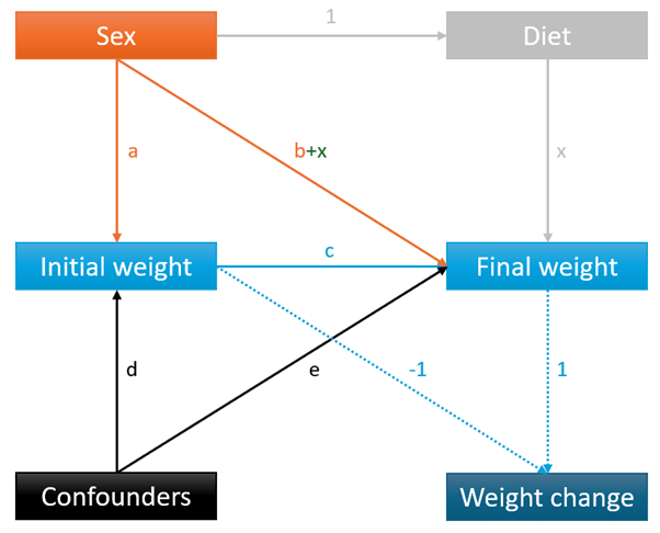
Anyway, the explanation of the DAG is this:

1. Arrows represent causation, and the absence of an arrow implies no causation, e.g. sex causes changes in initial weight, final weight, and diet, but not in confounders or weight change, except through initial and final weight
   • I use the word “variable” to refer to any of the words (sex, diet, etc.), while others use “nodes”
   • I use the words “exposure” and “outcome” to mean the variable at the start of the arrow (exposure) and the variable at the end of the arrow (outcome), so that the exposure always causes the outcome (others use different words, but these are the ones I find least confusing)
2. Any instance of 1 or -1 imply that the effect of the exposure on the outcome is 1 or -1: in this case, diet is completely determined by sex (all women have diet = 1, all men have diet = 2), and weight change is completely determined by final weight minus initial weight
   • We have to assume that there are 2 diets, one of which men have, the other of which women have
3. The other letters represent different effects of the exposures on the outcomes:
   • a = the effect of sex on initial weight
   • b = the effect of sex on final weight
   • c = the effect of initial weight on final weight
   • d = the effect of all confounders (of the initial weight-final weight relationship) on initial weight
   • e = the effect of all confounders (of the initial weight-final weight relationship) on final weight
4. To work out the contributions to variables, you add up the letters going into it, including indirect routes, which are multiplied
   • For example, final weight is determined directly by sex (b), initial weight (c), and confounders (e), but also sex through initial weight (ac), sex through diet (x), and confounders through initial weight (dc)
   • In practice, we’d use regression to work out what each letter was numerically. Adding different variables to the regression works out different letters and letter combinations
   • Note that letters represent direct effects, but regressions may give you total effects depending on the exposures and outcomes, for example:
     • if you regressed final weight on initial weight only, the coefficient for initial weight would be: c + ac + dc
     • if you regressed final weight on initial weight, sex, and confounders, the coefficient for initial weight would be: c
   • It’s all good fun, and why DAGs are so helpful – which letter are you actually trying to estimate, and what assumptions have you made to get there?

For absolute clarity, the only thing we want to know to answer the first research question is the effect of diet on final weight: x

Everything else doesn’t matter.

We want to know x.

For the second research question, we want to know if x is affected by sex.

But… We can’t know that. Ever. Even if we measured diet (which we didn’t), because men and women received entirely different diets.

Actually, we can’t know x either, because diet is completed subsumed by sex.

As such, the first DAG isn’t quite right, and this one probably works better:

Everything is the same, apart from the effect of diet on final weight is added to the effect of sex on final weight. Note that for our purposes, “Diet” doesn’t exist as a variable anymore: the effect of diet on final weight can’t be in 2 places at the same time, so now it’s just in the effect of sex on final weight.

This, I think, is the key distinction between how I’m thinking about this paradox, and how others have done (noting, again, this may be arrogant and fallacious).

Regression to the mean

Regression to the mean is a difficult concept, but my interpretation is this: continuous measurements (like weight) bounce around over time. This is often due to measurement error, but for weight, imagine also how much food and water someone had the day before, how much salt they had, whether they pooped before measurement, any sickness – the list goes on. The bouncing isn’t truly random – some elements are (like measurement error), but others are constrained and non-random: there is a limit to how much extra food someone can eat the day before, how long someone can go without food due to sickness, how much poop weighs, etc.

Overall, most people will have an average weight, which varies a little and randomly day-by-day.

If someone has a low (for them) initial weight, they are more likely to have a higher final weight: they ate more the day before, they weren’t sick, they hadn’t pooped that day, the scales randomly increased their weight, etc.

If someone has a high (for them) initial weight, they are more likely to have a lower final weight: they were sick this time, they were dehydrated, they pooped right before, the scales randomly reduced their weight, etc.

If someone had an initial weight that was bang-on their true average weight, then they are equally likely to have a lower or higher final weight.

In essence, regression to the mean can be interpreted as an attraction to the mean weight: low values are pulled toward higher values and vice versa. But because there’s a lot of randomness pushing and pulling, and there are more people with the mean weight and fewer people with extremely low or high weights, this all balances out at a group level (rather than everyone ending up with the mean weight at the end).

This means each person can change their weight, and they did: in the first graph, initial and final weights are drawn as ovals, indicating people changed their weight. If initial weight and final weight were the same for everyone, the ovals would be straight lines.

However, this also means that the distribution of weight in a population can remain the same: some people gain weight, some people lose it, some people stay the same weight, and it all evens out.

I would argue that regression to the mean is the most plausible explanation for having no weight change on average over time combined with everyone’s weight also changing over time.

Last thought before moving on

What does b mean here, the direct effect of sex on final weight?

How does sex affect final weight except through initial weight?

One answer would be sex differences in weight gain or loss over the university year.

That’s plausible, but:

1. there is no true weight gain or loss for men or women in the data (there may be other reasons for this, see below)
2. I wouldn’t intuitively expect university students to gain or lose weight naturally, that is, they’re not 10 years old and still growing.

However, another option for seeing no weight gain or loss for men or women is that there would have been systematic weight gain or loss for men or women, but there was an equal and opposite effect of confounding and/or diet that prevented this.

That is, people could have gained, say, 5% of their body weight over the year of the study. However, the university instituted an exercise regime that prevented it. Or the diet was so horrible the weight was never gained. Or everyone did gain the weight, but lost it all in the final week before the final weight measurement because of norovirus. Basically, something happened to counteract what would have been observed otherwise. Note that something could have been many things and affected men and women differently, but added up to no overall change in weight.

We can’t do anything about this, because we have insufficient data and it isn’t the most plausible explanation of what’s happening, so let’s assume that sex doesn’t affect final weight except through initial weight.

Ok let’s move on…

Actually, no, let’s not.

I did move on.

I wrote some simulations, and I wrote more blog, and then I had to come back and rewrite it.

Because while there is no direct effect of sex on final weight (b is 0), the total effect of sex on final weight is not 0.

There’s regression to the mean.

Let’s presume that sex affects true weight. That is, your average weight over, say, a month, when you weren’t gaining or losing weight. Each day might be different from this true weight, sometimes by a lot, but nonetheless you have a true weight.

Your true weight affects your initial and final weights, so the DAG (just for sex and weight) looks like this, assuming no weight change over time and no direct effect of sex on final weight (which would be weird, since sex already affects true weight):

So, when you regress final weight on initial weight and sex, would you expect to find an effect of sex on final weight?

Think about it for a minute.

…

…

…

The answer is: yes.

Why?

Because we haven’t measured true weight: the DAG for the regression actually looks like this (I’ve put the two exposures in the regression in black boxes):

Note: the effect of true weight on initial weight has been lost because we put initial weight into the regression, and this blocks on arrows going into it. I’ve also put the effect of initial weight on final weight as a dashed line, because there’s little evidence there would have been an increase in weight over time. I’ve put the effect of true weight on final weight as a blue and orange line, because there is an effect of true weight on final weight, but we didn’t measure true weight, so this effect looks like it’s from sex alone.

Sex does affect final weight: an indirect effect through true weight.

If you measured true weight and put that into the regression, then you’d correctly see no effect at all of sex on final weight.

Without this, though, you’ll see an effect of sex on final weight equal to the effect of sex on true weight multiplied by the effect of true weight on final weight.

I wrote a simulation to check this. It had 10,000,000 observations and was 50% male, 50% female. The results are precise, so I’m not going to give uncertainty (there is none).

In the simulation, I created a variable called true weight, which was a sex-specific normal distribution, with a mean of 60kg for women and 75kg for men, and a standard deviation of 2kg for each.

I then created initial and final weight, which were created by adding error to the true weight separately (normal distribution, mean of 0, standard deviation of 1). This added a little more variation to the weights (standard deviations now 2.24), but that’s fine. Also, it means initial weight does not cause final weight in any way: they are both derived from true weight, not from each other. They’ll still be highly correlated, but if I regress final weight on true weight and initial weight, there’d (correctly) be no effect of initial weight on true weight.

When regressing final weight on sex alone, being male adds 15kg, the average difference in weight for men and women. That’s correct.

When regressing final weight on initial weight alone, we see a coefficient of 0.98, interpreted as this: for every 1kg increase in initial weight, there would be a 0.98kg increase in final weight. The constant was also 1.1 kg, implying everyone gained 1.1kg between the initial and final weight measurements.

Weird, right? They definitely didn’t.

Why did this happen?

Because initial weight isn’t the only contribution to final weight: true weight also affects final weight.

The initial and final weight both have random error. The greater the random error relative to the standard deviation of true weight (as in, the greater the standard deviation of the error compared with the standard deviation of true weight), the lower the coefficient relating initial and final weights, and the higher the constant.

This doesn’t affect the coefficient of initial weight on final weight much here (0.98 vs the expected 1), but the coefficient gets substantially lower as the error increases relative to the standard deviation of the initial weight.

The constant, incidentally, has to be more than 0 if the relationship between initial weight and final weight isn’t perfect. The average initial and final weight are the same: 60kg for women, and 75kg for men. But since initial weight only has a coefficient of 0.98, that would mean the final weight would be, on average, lower than the initial weight. Everyone starting at 1.1kg negates this, and makes sure the means are the same for the initial and final weights.

Now, here’s where things get interesting.

When regressing final weight on initial weight and sex, the coefficients are, respectively, 0.80 and 3.00, with a constant of 12.

That is:

• every 1kg increase in initial weight increases final weight by 0.80kg
• being male adds 3kg to final weight
• everyone starts off at 12kg final weight

How, and why?

As above, initial weight is highly related to true weight, so there’s some association between initial and final weight. However, now that sex is included in the regression, the standard deviation of initial weight has dropped substantially (men and women having a 15kg mean difference in weight contributes hugely to the overall standard deviation of initial weight). This means the error is proportionately larger, reducing the coefficient for initial weight from 0.98 to 0.80.

Sex affects final weight entirely through true weight: the 3kg increase for men is entirely because of the effect of sex on true weight.

Everyone starts off at 12kg because of the imperfect relationship between initial weight and final weight, as above.

We can use the initial weight means to show how everything works out:

• women have a mean initial weight of 60kg: multiply this by 0.80 to get 48kg, then add 12kg to get a final weight of 60kg
• men have a mean initial weight of 75kg: multiply this by 0.80 to get 60kg, then add 3 kg to get 63 kg (for being male), then add 12kg to get a final weight of 75kg

I ran another simulation trying out different values of the difference in weight between men and women (between 0 and 20kg, in increments of 1kg), the standard deviation of weight (between 1 and 5kg), and the standard deviation of the error (between 1 and 5 kg).

The results showed that all the regression values were deterministic, and entirely based on:

• the variance of weight (standard deviation of weight squared)
• the variance of the error (standard deviation of the error squared)
• the mean initial weight of women
• the difference in weight between men and women

The coefficient for initial weight (how much initial weight is related to final weight):

(I imagine actual statisticians may have just known this, but whatever).

The coefficient for sex (how much being male adds to final weight):

The constant in the regression:

In summary, sex doesn’t directly affect final weight, but does indirectly affect final weight through true weight, which can’t be measured.

The degree to which sex affects final weight is dependent on the variance of the error, the variance of weight, and the mean difference in the weight of men and women.

I consider this to be the effect of regression to the mean, and it is very relevant to what statistician 2 does.

Back to the paradox

I think I’ve shown that we’re likely to see an effect of sex on final weight, even if one doesn’t exist, because we can’t measure true weight.

Let’s add in true weight to the complete DAG, and see what’s going on:

Crap, that’s complex.

Ok, let’s simplify things a little: let’s assume that there’s no direct effect of sex on final weight (I think this is plausible), that there is no confounding for the weight variables (this isn’t plausible, but that’s ok for now), and that there is no direct effect of initial weight on final weight (no change in weight over time, plausible), and see where that takes us:

Now, I haven’t seen a DAG like this before, where regression to the mean has been coded as a missing “true” variable, but it makes sense to me.

As ever, we want to know x.

The first statistician

The first statistician in the paradox concluded that: “there is no evidence of any interesting effect of the school diet (or of anything else) on student”, because there was no overall weight change.

Weight change can be worked out as a combination of all letters in the DAG (all direct and indirect paths):

Weight change = Final weight – initial weight

Weight change = [x + a] – [a] = x

So… Yes!

That works, assuming no effect of sex on final weight apart from through true weight, no natural change in weight over time, and no confounding of basically any of these variables.

Are these assumptions valid?

Nah, probably not (particularly the “no confounding” bit), but that’s not the point: with those assumptions, I think the conclusion of the first statistician is correct.

The second statistician

The second statistician in the paradox concluded that: “that the boys showed significantly more gain in weight than the girls when proper allowance is made for differences in initial weight between the two sexes”, because the constants in the sex-specific regressions accounting for initial weight were different.

Unlike the first statistician, I can’t find a way for the second statistician to be right about this.

I think the statistician effectively did this regression twice, once for men, and once for women:

The statistician then compared the constant terms in the two regressions.

I’m pretty certain that is identical to doing a regression with initial weight and sex, as above:

And we know from the above that the coefficient for sex will not be 0, even if there is no direct effect of sex on final weight.

There will be an effect of sex on final weight that goes through the unmeasured true weight.

There, almost by definition, must be regression to the mean for this data to make sense.

The second statistician adds: “When pressed to explain the meaning of this conclusion in more precise terms, he points out the following: If one selects on the basis of initial weight a subgroup of boys and a subgroup of girls having identical frequency distributions of initial weight, the relative position of the regression lines shows that the subgroup of boys is going to gain substantially more during the year than the subgroup of girls.”

Well, that’s regression to the mean, right there.

If we look at everyone who weighs 60kg initially, what do the final weights look like?

For women, 60kg is average, so around half will gain weight, and half will lose weight.

But for men, 60kg is 15kg below the mean. Almost all these men will gain weight.

So yes, looking at subgroups with “identical frequency distributions of initial weight”, men will gain relative to women, because the mean weight of women is less than that of men.

Paradox explained?

Maybe?

So many people have looked at this, and all come to separate conclusions, and I could be wrong about any of this!

Nonetheless, I’m going to go against what I’ve read and and conclude the following:

1. The first statistician is correct, for a given set of assumptions (some of which are plausible given the data, some of which are not)
2. The second statistician is incorrect, assuming there’s regression to the mean (which is the only way I can explain the data generated in the paradox)

I think regression to the mean explains the second statistician’s results entirely: the finding that men and women have different constants on regression is a consequence of sex affecting true weight, which is not measured but which causes both the initial and final weights (with error).

Notably, the first statistician doesn’t have issues with regression to the mean, because while weight change will be noisy thanks to measurement error, under the relevant assumptions, the effect of sex on final weight through true weight is offset entirely by the effect of sex on initial weight through true weight.

I ran an additional simulation for a sex difference in final weight due to different diets, and regressing weight change on sex gave the correct result for all different parameter values.

In short, weight change was correct given the assumptions made. Those assumptions could be wrong, in which case the result will be biased. Still, the second statistician is just plain wrong if there’s regression to the mean, and I’m convinced there must have been.

Overall, this paradox is paradoxical only in that at least one statistician is wrong: if you have repeated measures of a value, and that value has an underlying true value with measurement error, then a regression including an initial value and a variable affecting the true value will necessarily show an effect of that variable, even if none were present.

But the true answer to Lord’s research question is: this is stupid, do a trial or don’t use this data, either will be better.

Stata simulation code: *First simulation clear set obs 10000000 gen sex_difference = . gen sex_sd = . gen error_sd = . gen beta_weight_initial = . gen constant = . gen beta_weight_initial_adj = . gen beta_sex = . gen constant_adj = . gen sex = 0 replace sex = 1 in 1/5000000 gen weight_true = . gen weight_initial = . gen weight_final = . *Over different values of sex differences in weight, and standard deviations of weight and error, generate a true weight (from which initial and final weights are entirely derived), then: *1. regress final weight on initial weight and store the coefficient and constant *2. regress final weight on initial weight and sex, and store the initial weight and sex coefficients, and constant local i = 1 forvalues sex_difference = 0/20 {                 forvalues sex_sd = 1/5 {                                 forvalues error_sd = 1/5 {                                                 qui {                                                                 local weight = 60 + `sex_difference’                                                                 replace weight_true = rnormal(60,`sex_sd’) if sex == 0                                                                 replace weight_true = rnormal(`weight’,`sex_sd’) if sex == 1                                                                 replace weight_initial = weight_true + rnormal(0,`error_sd’)                                                                 replace weight_final = weight_true + rnormal(0,`error_sd’)                                                                 reg weight_final weight_initial                                                                 replace beta_weight_initial = _b[weight_initial] in `i’                                                                 replace constant = _b[_cons] in `i’                                                                 reg weight_final weight_initial sex                                                                 replace beta_weight_initial_adj = _b[weight_initial] in `i’                                                                 replace beta_sex = _b[sex] in `i’                                                                 replace constant_adj = _b[_cons] in `i’                                                                 replace sex_difference = `sex_difference’ in `i’                                                                 replace sex_sd = `sex_sd’ in `i’                                                                 replace error_sd = `error_sd’ in `i’                                                                 local i = `i’+1                                                 }                                 }                 } } *Keep only the results drop sex-weight_final keep if sex_sd != . *Generate estimates for the coefficients for initial weight and sex, and the constant, from the second regression gen est_beta_weight_adj = sex_sd^2/(sex_sd^2+error_sd^2) gen est_beta_sex = (1-est_beta_weight_adj)*sex_difference gen est_constant = (error_sd^2*60)/(sex_sd^2+error_sd^2) *These can be compared against the observed coefficients with regression, if necessary *Second simulation, as above, but with weight change as the outcome, and adding in a true effect of diet clear set obs 100000 gen diet_effect = . gen sex_difference = . gen sex_sd = . gen error_sd = . gen beta_weight_initial = . gen constant = . gen beta_sex = . gen constant_adj = . gen sex = 0 replace sex = 1 in 1/50000 gen weight_true = . gen weight_initial = . gen weight_final = . gen weight_difference = . *Over different values of sex differences in weight, and standard deviations of weight and error, generate a true weight (from which initial and final weights are entirely derived), then: *1. create a weight difference variable *2. regress weight difference on initial weight and store the coefficient and constant *3. regress weight difference on sex and store the sex coefficients and constant local i = 1 forvalues diet_effect = -5/5 {                 forvalues sex_difference = 0/20 {                                 forvalues sex_sd = 1/5 {                                                 forvalues error_sd = 1/5 {                                                                 qui {                                                                                 local weight = 60 + `sex_difference’                                                                                 replace weight_true = rnormal(60,`sex_sd’) if sex == 0                                                                                 replace weight_true = rnormal(`weight’,`sex_sd’) if sex == 1                                                                                 replace weight_initial = weight_true + rnormal(0,`error_sd’)                                                                                 replace weight_final = weight_true + rnormal(0,`error_sd’) + `diet_effect’*sex                                                                                 replace weight_difference = weight_final – weight_initial                                                                                 reg weight_difference weight_initial                                                                                 replace beta_weight_initial = _b[weight_initial] in `i’                                                                                 replace constant = _b[_cons] in `i’                                                                                 reg weight_difference sex                                                                                 replace beta_sex = _b[sex] in `i’                                                                                 replace constant_adj = _b[_cons] in `i’                                                                                 replace diet_effect = `diet_effect’ in `i’                                                                                 replace sex_difference = `sex_difference’ in `i’                                                                                 replace sex_sd = `sex_sd’ in `i’                                                                                 replace error_sd = `error_sd’ in `i’                                                                                 local i = `i’+1                                                                 }                                                 }                                 }                 } } drop sex-weight_final keep if sex_sd != . *Check if the sex coefficient is equal to the diet effect reg diet_effect beta_sex